On the fundamentals of gradient-based SAT solvers

At NeurIPS 2026 in Sydney, we will be presenting our paper On the fundamentals of gradient-based SAT solvers. I will give a brief overview of the formulation and three questions that guide our study: how initialization affects convergence, how symmetries interact with neural parametrization, and how formula transformations change the optimization problem.

Continuous SAT solving and extensions

Boolean satisfiability (SAT) asks whether we can assign true or false to variables so that a formula is satisfied. In conjunctive normal form (CNF), the formula is an AND of clauses, each an OR of variables or their negations. We focus on Max-SAT, or equivalently Min-UNSAT, where the goal is to satisfy as many clauses as possible. A satisfiable formula has a minimum of zero violated clauses.

There has been a rise in interest in SAT solvers based on continuous local search since methods like FourierSAT and GradSAT have shown promising results on certain challenging problems, including instances with cardinality and pseudo-Boolean constraints. The key idea behind these methods is to write down a continuous formulation of the SAT problem and use a variant of gradient descent to reduce the number of violated clauses. There is no unique or right way to do this, but one formulation comes from the multilinear extension.

Let \(\Phi\) be a CNF formula on \(n\) Boolean variables \(x_1,\ldots,x_n\), viewed as a set of clauses. For an assignment \(x\in\{0,1\}^n\), let \(V_\Phi(x)\) count the violated clauses and write \(C(x)=0\) when clause \(C\in\Phi\) is violated. We also write \(\Phi(x)=0\) when \(x\) fails to satisfy the formula. Assign variable \(x_i\) a probability \(p_i\) of being true. That means we have a vector of probabilities \(p=(p_1,\ldots,p_n)\) for all variables. Let \(X\sim\mu_p\) denote the random assignment obtained by sampling the variables independently. Taking the expectation gives

\[\mathcal{L}_\Phi(p) = \mathbb{E}_{X\sim\mu_p}[V_\Phi(X)] = \sum_{C\in\Phi}\Pr_{X\sim\mu_p}[C(X)=0].\]

This is easy to evaluate and differentiate. For example, the probability of violating the clause \(x_1\vee\neg x_2\) is simply \((1-p_1)p_2\). It is also the loss obtained by applying the probabilistic approach from my earlier Erdős Goes Neural paper to SAT. The expected number of violated clauses provides an upper bound on the probability that any constraint is violated.

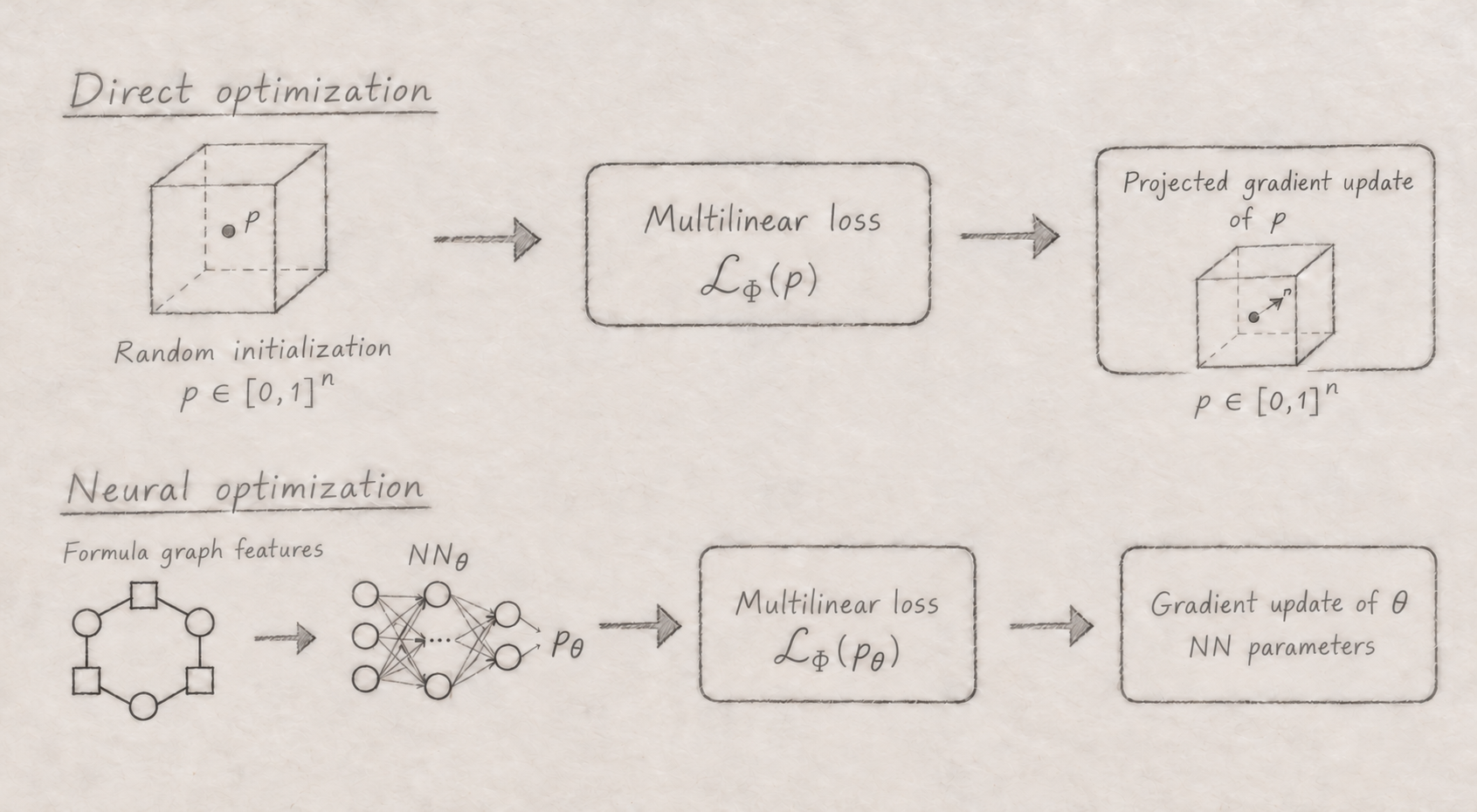
\[\Pr_{X\sim\mu_p}[\Phi(X)=0] = \Pr_{X\sim\mu_p}\!\left[\bigcup_{C\in\Phi}\{C(X)=0\}\right] \le \sum_{C\in\Phi}\Pr_{X\sim\mu_p}[C(X)=0].\]

For CNF formulas, this objective is essentially equivalent to the sum of the clausewise Walsh–Fourier expansions used in continuous SAT solvers (up to constants/rescaling). This connects the expectation-based loss to first-order optimization of Fourier objectives. We can optimize the probabilities directly or produce them with a neural network and optimize its parameters (see figure).

This probabilistic perspective also helps us think about optimization. For unsatisfiable formulas, minimizing this bound can be more effective than maximizing the exact probability of satisfaction, even setting computational cost aside (can you see why?).

With this common formulation, we study three issues that have also been investigated for discrete solvers.

1. Convergence properties and initialization

We first study how the initialization affects whether projected gradient descent reaches zero expected violations. A formula requiring exactly one of three variables to be true provides a simple example of this difficulty. Its satisfying assignments are \((1,0,0)\), \((0,1,0)\), and \((0,0,1)\). If we initialize with \(p_1=p_2=p_3\), symmetry makes the three gradients equal, so every update preserves that equality. The subspace defined by \(p_1=p_2=p_3\) is therefore an invariant subspace that gradient descent cannot leave. The optimization remains in a subspace containing no zero-loss solution, even though the formula is satisfiable. We derive sufficient conditions that instead guarantee convergence to zero loss, identifying successful initializations for structured formula families. For the exactly-one example, suitable asymmetric initializations can satisfy these conditions and converge to a one-hot solution.

2. Symmetries and neural parametrization

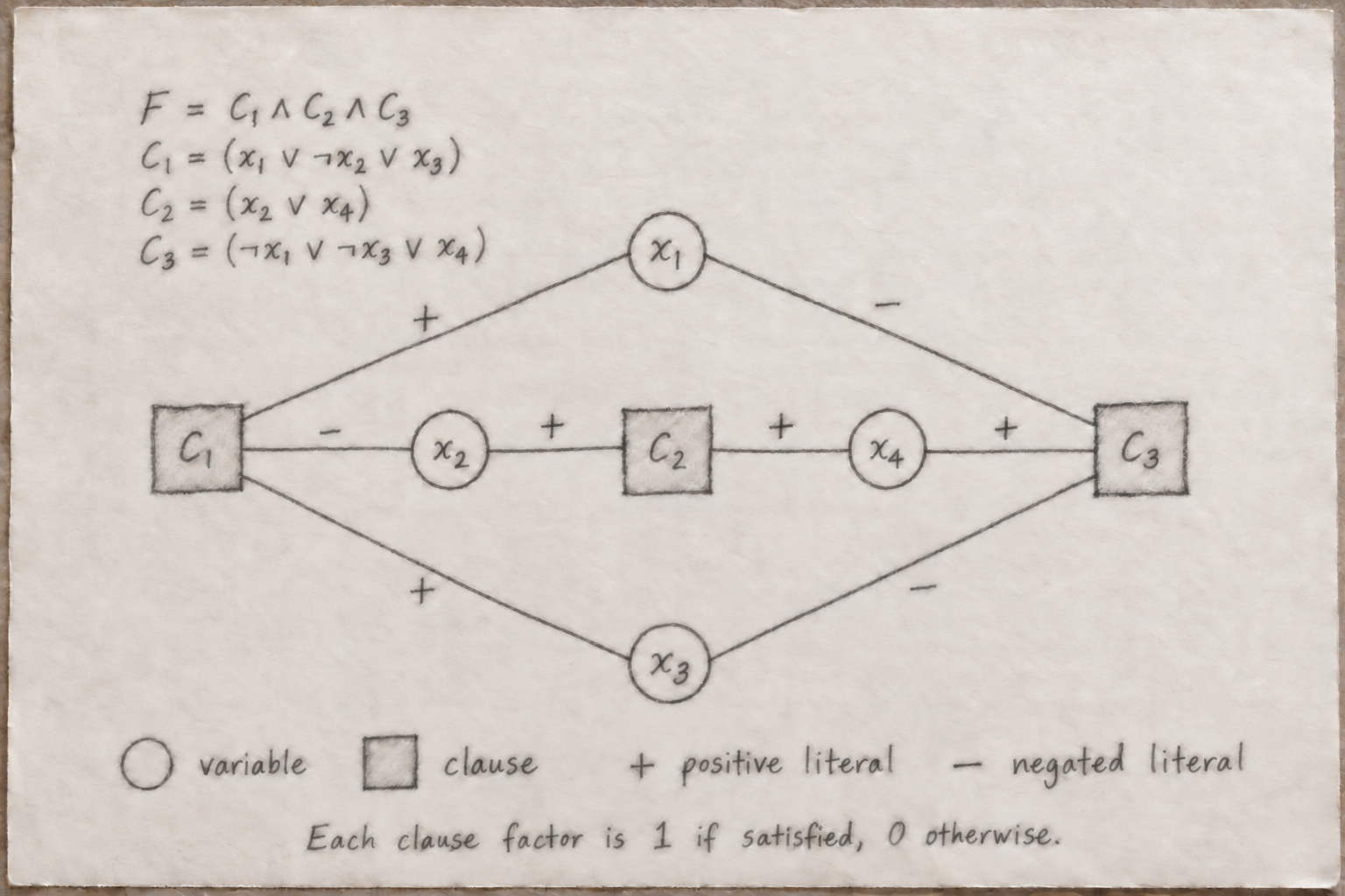
The symmetry in the exactly-one example is part of a more general phenomenon. We can represent a formula as a signed variable–clause graph, with one node per variable and clause, and signed edges recording positive or negated occurrences. To compare nodes, we start with separate colors for variables and clauses, then repeatedly refine these colors using the number of neighbors of each color and edge sign. Once no more groups split, the remaining groups are stable color classes. Nodes in the same class are indistinguishable under this refinement.

We show that these stable color classes define invariant subspaces for gradient descent. If variables in the same color class start with equal probabilities, gradient descent keeps those probabilities equal throughout optimization.¹ When every satisfying assignment requires breaking that equality, this prevents convergence to zero loss. Color classes also give us a similar result for neural solvers. A 1-WL-style message-passing GNN with shared updates and no distinguishing input features or node identifiers assigns identical outputs to variables in the same stable color class, for every choice of network parameters.

3. Formula transformations

Finally, we study familiar SAT operations such as unit clause propagation, resolution, and variable elimination. These preserve satisfiability, but they can change the continuous loss, its smoothness, and the graph seen by a neural network. For example, adding a logically redundant clause leaves every satisfying assignment unchanged while adding a new term to the expected-violation objective. The exact probability of satisfaction at fixed \(p\) is unchanged, but the new term can alter the optimization trajectory and, on satisfiable instances, change the probability of sampling a satisfying assignment from the final marginals. We analyze these effects and show that certain transformations can also break expressivity barriers of message-passing GNNs. We see that simplifications such as unit propagation can help direct gradient descent, while transformed instances can improve data efficiency and inference-time performance for self-supervised neural solvers. The representation of a formula is therefore part of the algorithmic design, with consequences for both the optimization dynamics and the capabilities of neural solvers.