Learning with Neural Extensions

This post is meant to serve as an intuitive and practical explainer of our work on neural set function extensions, recently presented at NeurIPS 2022. As in previous posts, I will be skipping potentially important details in the interest of brevity and accessibility. Throughout the text, I will be making an effort to accommodate the non-expert reader. This might make the text a bit tedious or repetitive for the people already familiar with this kind of setting, so feel free to skim through the boring parts if that’s you. Now, let’s get started.

Motivation

Neural networks natively operate in continuous domains, where we can update their parameters through gradient-based optimization. However, many problems that we care about solving are defined over discrete domains and their solutions often involve different kinds of discrete computation. These may be algorithmic tasks like sorting numbers or finding shortest paths on graphs, or maybe playing games like chess and Go. Applying neural networks to discrete domains/tasks can lead to the discovery of new effective algorithms for those problems but at the same time it comes with its own set of challenges. Discrete representations and operations introduce discontinuities and non-differentiabilities in end to end pipelines. Our paper is another step towards overcoming some of the incompatibilities between neural networks and discrete computation.

Zooming in a bit more, a general problem that is commonly found in machine learning is that of picking an object or a set of objects that is the best with respect to a certain criterion. For example, in image classification, we predict some labels and the criterion we care about is whether the predicted labels match the true labels of the data. In strategy games, we often have a discrete space of actions and the criterion is some reward defined over the action space. In combinatorial optimization, we have a discrete space of possible configurations of objects and we are interested in the configuration that minimizes an objective function. In all of those cases, there is a function defined on a discrete space (space of labels, space of actions, space of configurations) which evaluates the quality of the discrete input that is provided. However, neural networks produce continuous representations which are incompatible with such functions. Furthermore, such discrete functions aren’t necessarily differentiable either, so we can’t directly use them as the loss function of our neural network. To solve such problems with NNs, we use continuous and differentiable proxies in place of the original function as a training loss. In classification, we use the cross-entropy as a loss function, which acts as a proxy for the training accuracy. If we want to evaluate how well we are doing in terms of accuracy in a classification task, we may perform a discretization step (e.g., argmax) of the continuous output. If there isn’t a known differentiable proxy for the function we care about, we may treat the function as a black-box and optimize it directly using reinforcement learning algorithms. In that case, discretization happens generally by sampling discrete representations from the continuous output of the neural network.

In our paper on set function extensions we propose an alternative that deals both discrete domain of functions as well as their differentiability. We show how to create continuous and differentiable extensions (proxies) of discrete functions, i.e., functions compatible with continuous inputs (e.g., outputs of neural networks) that we can backpropagate through in neural network pipelines. In fact, many of our extensions enable this in a completely black-box manner, i.e., without requiring a closed form expression for the discrete function. Furthermore, drawing inspiration from semidefinite programming as well as more recent work in the ML community on neural algorithmic reasoning and knowledge graph reasoning, we show how to extend discrete domains to higher dimensions so that discrete functions can be applied directly to high-dimensional embeddings. This post will focus on the low-dimensional case; extensions onto high-dimensional spaces will be discussed in part 2 of this post.

A more concrete example and possible approaches

Suppose that you have a neural network which produces a score vector \(\mathbf{x} \in [0,1]^{n}\) given some input problem instance (a graph, an image, etc.), which is then used to solve some downstream task. That vector could be marginal probabilities of graph nodes for some kind of node selection task, or even the class probabilities for a classification task. To make the presentation more concrete, we will treat \(\mathbf{x}\) as marginal probabilities for node selection, i.e., \(x_i\) is the probability that node \(i\) belongs to a set of nodes \(S\) that is meant to solve some graph problem (a set that optimizes some kind of objective function).

Now assume that you have a function \(f: 2^n \rightarrow \mathbb{R}\) whose input is any subset of \(n\) items. We can view the domain of \(f\) as the space of n-dimensional binary vectors, i.e., \(f: \{0,1\}^n \rightarrow \mathbb{R}\). I’m obviously abusing notation here to emphasize that the inputs of this function are discrete, however the outputs are allowed to be continuous. Throughout the text I will be using notation for sets and binary vectors interchangeably. The input domain consists of all the possible indicator vectors for all the subsets of \(n\) items we could pick. For instance, let’s assume \(f\) is the cardinality function, i.e., the function that counts how many items the provided set has. Then for \(n=3\), a set \(S\) could be represented by a 3-dimensional binary vector, e.g., \(\mathbf{1}_S= \begin{bmatrix}1 & 1 & 0 \end{bmatrix}\). In the case of that example vector, clearly the cardinality is \(f(S) = f(\mathbf{1}_S) = 2\).

Naturally, that kind of function is not compatible with arbitrary \(\mathbf{x}\) due to the continuity of \(\mathbf{x}\). For instance, it doesn’t make much sense to ask what is the cardinality of \(\begin{bmatrix} 0.3 & 0.5 & 0.2 \end{bmatrix}\) to begin with. If we want to find a set that minimizes (or maximizes) the function by improving the scores in \(\mathbf{x}\) in a differentiable neural network pipeline, we have to square away this incompatibility. Here, there are certain options one would consider:

Discretize the continuous output. We could sample with the Gumbel trick or even just threshold the values of \(\mathbf{x}\) to obtain a binary vector that represents a set. We could then use a straight-through estimator in the backward pass to go through the discretization procedure. While this provides a discrete vector that \(f\) is compatible with, it may only work if the function \(f\) itself is differentiable.
There will be plenty of cases where \(f\) is given as a black box, so we have no guarantees that we can differentiate through it. In that case, some kind of stochastic gradient estimation might be our next option. For example we could use REINFORCE, i.e., sample sets \(S\) from \(\mathbf{x}\) then use the log-derivative trick to backpropagate through \(\mathbf{x}\) while treating \(f\) as the reward function.
Use a known continuous relaxation of the function. Again, that assumes that we have access to the function and a bespoke relaxation exists. That does not require any discretization as the relaxation by definition accepts continuous inputs. When available, this can be a pretty good option. In the case of the cardinality function, one has to add all the elements of the binary vector to obtain the cardinality of the set. In other words, \(f(\mathbf{1}_S)= \sum_{i=1}^n \mathbb{I}_{i \in S}\). Here, \(\mathbb{I}_{i \in S}\) returns 1 if \(i \in S\) and 0 otherwise. This can be naturally relaxed in the \([0,1]^n\) interval by taking \(\bar{f}(\mathbf{x}) = \sum_{i=1}^n x_i.\) This is great but it can only be done if we have a closed form expression for the function. In the case where the function is a black-box, we’re out of luck.

Our solution

These are all valid strategies that could make sense in certain scenarios. Here, we will propose an alternative that aims to mitigate the drawbacks of the aforementioned apporoaches. First, we can go back to the main obstacle we started from. What does it mean to ask about the cardinality of the input (value of the discrete function) when the input is not a set (binary vector) but a vector of continuous values? There is a way to make this question well-posed. We can treat the continuous values as parameters of a probability distribution over sets. Then we can ask what is the expected value of the function over the distribution of sets encoded by \(\mathbf{x}\).

What is a scalar set function extension? It is simply a new differentiable function \(\mathfrak{F}: [0,1]^n \rightarrow \mathbb{R}\) which extends the discrete domain of the original function to a continuous domain. We will define it as a weighted combination of evaluations of the original function at discrete points, or equivalently, as the expected value of the function \(f\) over a distribution of sets encoded by \(\mathbf{x}\).

image description

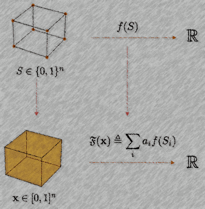
That means that we will be going from a function defined on the corners of the hypercube \(\{0,1\}^n\) to a function defined on the whole hypercube \([0,1]^n\). We propose continuous and differentiable extensions of discrete functions defined on sets, that can be deterministically computed, even when we’re only given black-box access to \(f\). We provide multiple extensions that originate from a common mathematical formulation. Some are already known like the Lovász extension, and others are new, like the bounded cardinality Lovász extension.

Scalar extensions explained

We call \(\mathfrak{F}\) a scalar extension of a function \(f\), if \(\mathfrak{F}(\mathbf{1}_S) = f(S)\) for all \(S\) in the domain of \(f\). For example, \(\mathfrak{F}(\mathbf{0}) = f(\emptyset)\), i.e., the extension evaluated at the origin (all-zeros vector) should correspond to \(f\) being evaluated at the empty set.

How can you compute \(\mathfrak{F}\)?

There is a simple trick to defining \(\mathfrak{F}\). As explained earlier, we can view \(\mathbf{x}\) as encoding a distribution over sets. To do this, we can express any continuous point in the n-hypercube \(\mathbf{x} \in [0,1]^n\) in the following way:

\(\displaystyle \mathbf{x} = \sum_{i} a_i \mathbf{1}_{S_i}, \quad \displaystyle \sum_i a_i = 1, \quad a_i \geq 0.\)

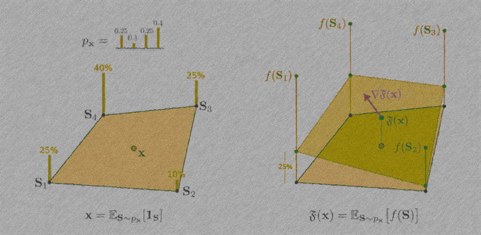
In other words, for every continuous point in the hypercube, we can find certain corners of the hypercube and express said point as a convex combination of those corners. This defines a distribution:

\(\mathbf{x} = \displaystyle\mathbb{E}_{S \sim \mathbf{p_x}}[S]\).

Here \(\mathbf{p_x}\) is the probability distribution induced by \(\mathbf{x}\). This distribution is fully described by the coefficients \(a_i\) in the convex combination. Once we have \(S_i\) and \(a_i\) defining \(\mathfrak{F}\) is simple:

\(\mathfrak{F}(\mathbf{x}) \triangleq \displaystyle\sum_{i} a_i f({S_i}) = \mathbb{E}_{S \sim \mathbf{p_x}}[f(S)]\).

The distribution is supported only on sets \(S_i\) and each set has a corresponding probability of \(a_i\). Intuitively, the value of the extension at the continuous point is just a weighted combination of the values of the original function \(f\) at the corners that form the convex combination of \(\mathbf{x}\). Furthermore, the weights of the weighted combination are precisely the same weights used to express \(\mathbf{x}\) as a convex combination of hypercube corners.

A large chunk of the paper is dedicated to properly formalizing this trick. Obviously, I will keep things simple here so I won’t get into all that. I encourage the curious reader to check out the paper. Now, there are a couple of questions that naturally have to be addressed. One has to do with how we find those sets \(S_i\) and their coefficients \(a_i\). Is it computationally tractable? Can we do it fast? The other has to do with whether this thing is differentiable at all. The answer to all those questions is, modulo certain disclaimers, yes. (Note that by ‘differentiable’ I will only be referring to differentiability in the sense that we can use automatic differentiation with packages like Pytorch and Tensorflow. Check out the appendix of the paper for more detailed comments around that.)

How can we backpropagate through \(\mathfrak{F}(\mathbf{x})\)?

The trick for this is simple. As long as \(a_i = g(\mathbf{x})\), and \(g\) is some differentiable function of \(\mathbf{x}\), then gradients can just go through the coefficients \(a_i\) in the sum that defines \(\mathfrak{F}(\mathbf{x})\). (The coefficients) image description

How do we find sets \(S_i\) and their coefficients \(a_i\)?

In the paper we provide multiple examples of scalar extensions. Each one comes with its own way of computing sets \(S_i\) and their probabilities \(a_i\). Crucially, the coefficients \(a_i\) depend continuously on \(\mathbf{x}\) which allows us to do backpropagation. The ‘cheapest’ extensions that require only black-box access to the function \(f\) are the Lovász extension, the bounded-cardinality Lovász extension, the singleton, and the permutation/involutory extensions. These all require \(n+1\) sets (including the empty set) and coefficients. Before I go into specific extensions and how to compute them, I want to emphasize that the key point to remember is that you could find your own extensions by figuring out ways to express continuous points as convex combinations of discrete points. I may discuss some general strategies for this in a future post but for now I will just leave it at that.

In practice: The Lovász extension

The Lovász extension is well known in the fields of discrete analysis/optimization and submodularity. It has various particularly nice properties but perhaps the most important one is that iff \(f\) is a submodular function, then the Lovász extension of \(f\) is convex. Examples of submodular functions include graph cuts, coverage functions, rank functions, and so on. Computing the Lovász extension is straightforward. First, we index the entries of \(\mathbf{x}\) in sorted, decreasing order: \(x_i \geq x_{i+1}\) for \(i=1,2,\dots , n-1\). That means that \(x_1\) corresponds to the dimension with the largest entry in \(\mathbf{x}\), \(x_2\) to the second largest, and so on. The coefficients and the sets of the Lovász extension are then defined as follows:

\(a_i = x_i - x_{i+1}\)

\(S_i = \{1:i \}\).

Here, I’m using a bit of coding notation with \(1:i\) to indicate “all elements up to \(i\)”. Given the sets and their coefficients, the Lovász extension is computed by

\(\mathfrak{F}(\mathbf{x}) = \displaystyle \sum_{i=1}^{n} (x_i - x_{i+1})f( \{1: i \} )\).

Clearly, \(a_i\) are differentiable with respect to \(\mathbf{x}\) as they’re just pairwise differences of the coordinates of \(\mathbf{x}\) To make things concrete, let’s do the calculation to find sets and coefficients for our example vector from before: \(\mathbf{x} = \begin{bmatrix} 0.3 & 0.5 & 0.2\end{bmatrix}\). Based on the ranking of the elements, we will have the following sets

\(1_{S_1} = \begin{bmatrix} 0 & 1 & 0 \end{bmatrix}, 1_{S_2} = \begin{bmatrix} 1 & 1 & 0 \end{bmatrix}, 1_{S_3} = \begin{bmatrix} 1 & 1 & 1 \end{bmatrix}\),

and the following coefficients

\(a_1 = 0.5-0.3 = 0.2,\)

\(a_2 = 0.3-0.2 = 0.1,\)

\(a_3 = 0.2\) .

It is easy to verify that \(\mathbf{x} = \sum_{i} a_i \mathbf{1}_{S_i}\). One might notice that \(\sum_i a_i <1\) in this case, even though I initially said that we need a sum to one. Thankfully, that’s not a problem because we can allocate the remaining probability mass to the empty set. By convention \(f(\emptyset) = 0\) so that term just cancels out. Therefore, we don’t strictly need the sum to 1, \(\sum_i a_i \leq 1\) can also be fine.

Converting discrete objectives to loss functions for combinatorial optimization and beyond

A standard use case for extensions in practice is when we have some kind of quantity of interest that is defined over sets of objects and we would like to find a set that optimizes it. This is a sufficiently general setting that could encompass graph and combinatorial problems, classification problems, NLP problems, etc. Extensions can let us do that by finding the continuous version of that quantity through \(\mathfrak{F}\) and then backpropagating to find representations that optimize it.

Combinatorial objectives

Let’s look at a simple application of extensions to combinatorial optimization. Consider the graph cut function. It is a submodular set function, that given a set \(S\) of nodes in an input graph \(G\), it counts the number of edges that have one endpoint inside \(S\) and one endpoint outside of \(S\) in the graph. It is known that finding a set that maximizes the graph cut is an NP-Hard problem. Minimizing it is by default in P (can you guess why?) but adding a simple cardinality constraint can make minimization NP-Hard as well. A way to tackle the problem of optimizing the cut (either min or max) could be to provide a graph instance on \(n\) nodes to a neural network and then generate some scores for the nodes of the graph \(\mathbf{x} \in [0,1]^n\). That’s where the extensions come in. Here we can use the extension of the graph cut function as a loss function to optimize. Then we can backpropagate through the neural network scores \(\mathbf{x}\) and update the parameters of the network. Normally, that wouldn’t be possible because we wouldn’t be able to backpropagate through an arbitrary set function. Now, the graph cut function happens to admit numerous continuous relaxations that are well known. One of those is the graph total variation \(TV(\mathbf{x};G) = \displaystyle\sum_{(x_i>x_j)} (x_i-x_j)w_{i,j}\), where \(w_{i,j}\) is the weight for any edge \((i,j)\) in the graph \(G\). It turns out that the Lovász Extension of the graph cut function is precisely the TV function so this is a case where a bespoke relaxation is naturally absorbed in our framework.

However, the same trick could be done for any other combinatorial problem. Take its objective function \(g(S)\) and a function that encodes the constraint \(c(S)\). For instance, for the maximum clique problem, \(g(S)\) is the number of nodes of \(S\), which we seek to maximize. The constraint \(c(S)\) on the other hand can just be a binary signal, it can be defined as follows:

\(c(S) = \begin{cases} 1 \; \text{if the set is a clique,} \\ 0 \; \text{ otherwise.} \end{cases}\)

Then we may combine \(c\) and \(g\) into \(f(S) = c(S)g(S)\). This is now a discrete set function which we can attempt to maximize in order to solve the maximum clique problem. We compute its continuous extension and use that as a loss function in order to find a score vector \(\mathbf{x}\) that encodes a distribution of sets \(S\) that best solves the problem.

Putting it all together: A recipe for solving problems with extensions

To summarize, here are 4 steps to start solving problems with extensions. Assuming you have some discrete function \(f: \{0,1\}^n \rightarrow \mathbb{R}\) and you are looking for subsets of \(n\) objects that give you the optimal value for that function.

Step 1: Get a neural network and an input instance (image, graph, whatever).
Step 2: Generate scores \(\mathbf{x} \in [0,1]^n\). The dimension \(n\) may be the number of nodes of a graph, the number of classes for classification, etc.
Step 3: Compute an extension \(\mathfrak{F}\) of the function \(f\). Use \(\mathfrak{F}\) (with an appropriate sign for minimization/maximization) as your loss function.
Step 4: To decide on a set for the solution to the problem, generate the sets \(S\) of the extension and pick whichever gives you the best value for \(f\).

That’s pretty much it. In the paper we apply those steps to do combinatorial optimization but we also show how they can be used for image classification by defining an extension for the discrete training error function (the possible input subsets there are just the \(n\) possible class labels that are represented by one-hot binary vectors). From brief discussions I’ve had at NeurIPS 2022, it seems like this kind of trick could be applied to other settings like NLP or VAEs. Those applications are left as an exercise to the reader :)

Conclusion and Part 2: Neural Extensions

To conclude, apart from using extensions as loss functions, we may incorporate them at other parts of end-to-end pipelines. For example, we could compute structural attributes of node neighborhoods in a graph using set functions, and then use those attributes as node features for a GNN that solves some downstream task. Extensions would allow us to backpropagate through the computation of those input attributes. I am obviously speculating here, but the bottom line is that apart from being used as loss functions, extensions could serve other purposes in an end-to-end pipeline.

Finally, this post has dealt with the first half of the paper. You may have noticed that I avoided discussing the meaning of the word scalar in the subtitle of the post. The characterization of scalar set function extensions has to do with the domain of the extension. If the extensions work on the hypercube like \(\{0,1\}^n \rightarrow [0,1]^n\), we are assigning a single scalar continuous score to each item among \(n\) items. In part 2 of this series, we will see how we can stretch the definition of extensions to allow for extensions of the form \(\{0,1\}^n \rightarrow [0,1]^{n \times d}\), i.e., \(d\)-dimensional embeddings for each item, which is usually the kind of representation that the layers of a neural network operate with (\(d\) would just be the width of a NN). But that’s a story for another time. Until then, I hope this has been helpful.

Nikos Karalias